Overview

GLOSSARY

KPI	Key Performance Indicator, also used as a generic term for visualisation components on a dashboard (e.g. Dial, Gauge, Status Indicator etc.)
Tag	An industry term for the name (or ID) of the timeseries data for a sensor in a data historian. All equipment in a facility is “tagged” with a unique identifier, and these unique identifiers are commonly referred to as “tags”.

1 Overview of Calculations

1.1 What are Calculations

Calculations apply “in-line” transforms to any timeseries data source connected to Ingenuity. Anything from simple mathematical operators such as Add, Subtract, Multiply and Divide, through more complex Totalisers and statistical functions like Average and Standard Deviation, logical If..Then functions and complex transforms such as Timeshifting.

Calculations can be nested, and multiple transforms can be applied sequentially.

The output of a Calculation is a Virtual or Synthetic timeseries that can be used in the Ingenuity in exactly the same way other Timeseries sources.

Unlike most of the other modules in Ingenuity, the Calculations module is not shown in the left hand panel because it behaves as a Historian datasource. It is accessible from any component that can take a Historian datasource.

1.2 What are Virtual Timeseries?

Virtual timeseries behave exactly like ‘normal’ (i.e. real or raw) signals stored as tags in process data historians but they are evaluated only when they are called. They can be used in exactly the same way as normal historian tags in Ingenuity.

For example, you can set limits & alerts or use as the basis for another virtual timeseries, but they are evaluated at runtime and do not need the values to be written back to a database.

The advantage of this is that they can be immediately plotted for any time period for which the source data exists, but they do not fill up storage space.

This allows experimentation and quick calculations for analysis without worrying about filling up memory or waiting until historical values are recalculated.

Virtual timeseries can be nested and multiple different functions combined in a single timeseries to produce complex calculations.

1.2.1 Example — unit conversion

If a pressure is measured in ‘bara’ but is required in ‘psia’ then it must be transformed by multiplying it by 14.5. If the source tag is called “Pressure-123” then the calculation would be:

calc/MUL(Pressure-123, 14.5)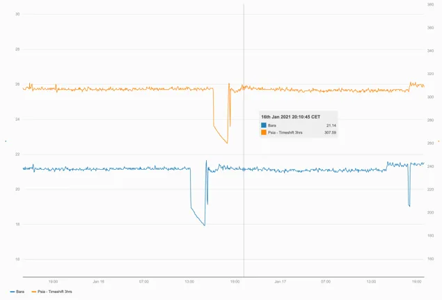

The orange series is a virtual timeseries created by multiplying the original tag (blue) in ‘Bara’ by 14.5 to get ‘Psia’ and then timeshifting the results by 3 hours forwards.

1.3 Creating Calculations (accessing the Editor)

The Calculation graphical editor is on the “Calculation” tab in the “Edit tag” form.

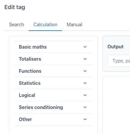
This form appears when the “Add tag” button is clicked on a trend:

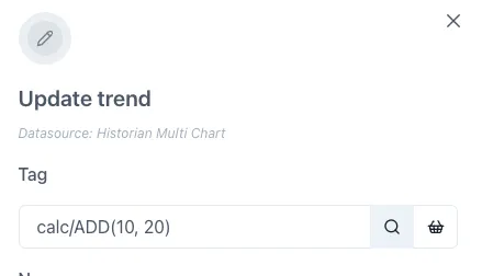
Or when the magnifying glass icon is clicked on the right hand side of the tag datasource entry field when editing a tag on a trend or dashboard:

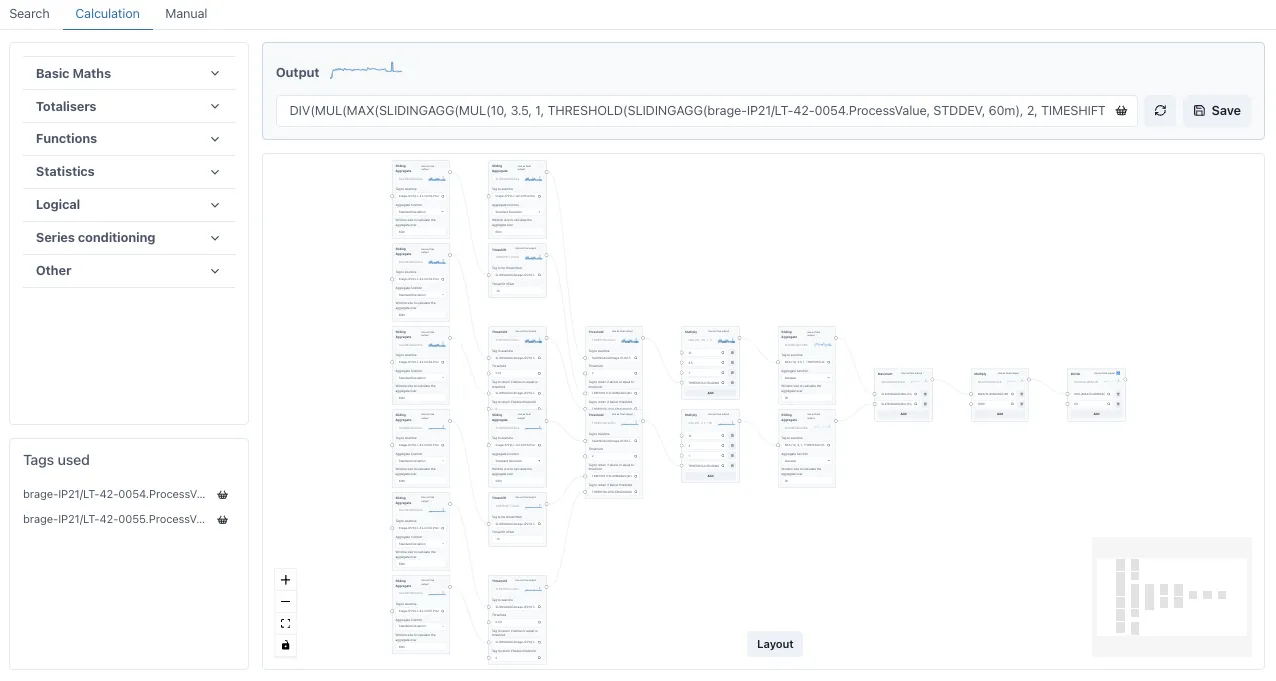
1.4 Editing the Calculation Equations

Ingenuity 7’s virtual calculation graphical editor is an easy-to-use drag-and-drop user interface in which any Ingenuity user can quickly configure complex calculations while minimizing human error.

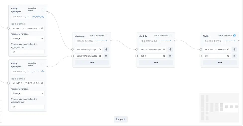
Transform function blocks are dragged and dropped into a canvas, after which inputs and outputs can be connected to compose any complex transformation.

Calculations can be linked together to form complex expressions multiple layers deep and the performance remains fast.

The extract below is from a function that calculates chemical dosing based on tank level changes.

1.5 Example use cases

1.5.1 Smoothing noisy signals

Averages can be applied to smooth out noisy signals

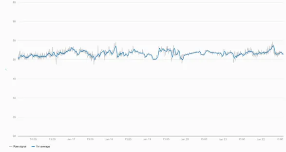
By applying an averaging function with a 1-hour window the underlying trends in the data can be seen more easily.

1.5.2 Logical expressions

The green series in the trend below uses the Threshold function to create a virtual timeseries of the flow only when Pump B is running.

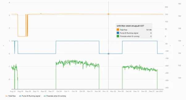
By using a Threshold function to only display the flowrate if the running signal is >0.5, a virtual timeseries is created that could drive a virtual flowmeter graphic.

1.5.3 Totaliser

Using the Totaliser function allows a value to be totalised over any window from 1 minute to years.

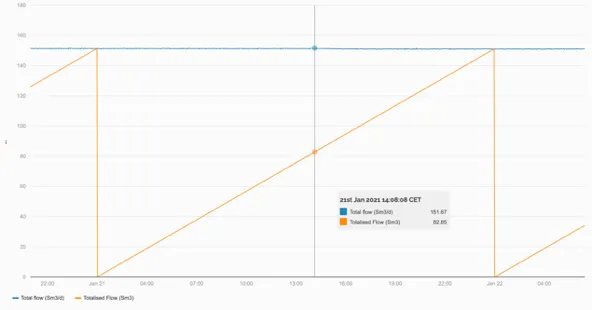
A flowrate in Sm3/d is totalised over 24hrs starting at midnight, giving the cumulative flow so far in any given day (orange line).

1.5.4 Combining two functions

Combining a Totaliser function with a Threshold function we can combine the two examples above to see the total amount of fluid pumped by Pump B in a year.

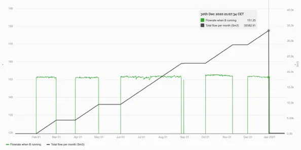
The virtual timeseries of the flow through Pump B is totalised in a second virtual timeseries over a window of a year starting at midnight on the 1^st January.

1.5.5 Taking the Maximum of several tags

The Max function lets users create a virtual timeseries that only shows the maximum value at any time from two or more tags.

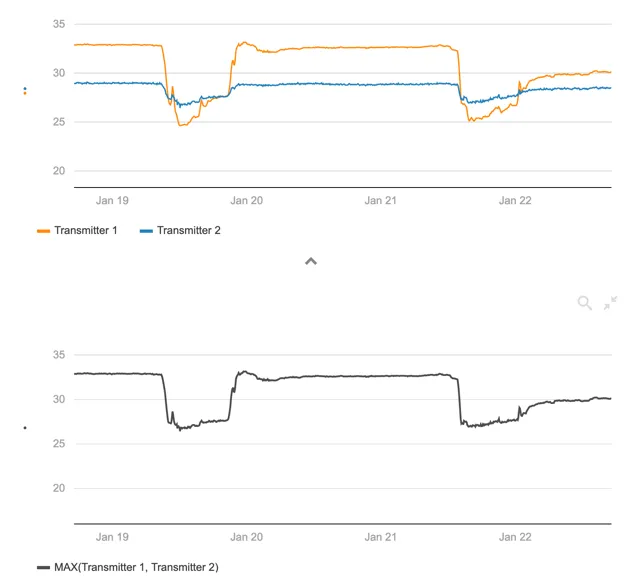
The upper trend shows the readings from two different transmitters. Using the Max function, we are able to create a virtual timeseries (lower trend — black line) that always shows the maximum reading from either of these two transmitters.