Calculations Details

2.6 Basic Maths

2.6.1 Add, Subtract, Multiply, Divide

These functions take a list of inputs separated by commas. The syntax for the Basic Maths functions ADD, SUB, MUL and DIV is:

ADD(a, b,..., n)

SUB(a, b,..., n)

MUL(a, b,..., n)

DIV(a, b,..., n)

a, b,.. n — any valid timeseries input (see section 2.2)

The inputs are processed from right to left which means that the SUB and DIV functions will return different results depending on the order of the inputs:

DIV(10, 8) = 1.25

DIV(8, 10) = 0.8

2.6.2 Percent Deviation

This function returns the percent deviation of input b from input a. The syntax for the PERCENTDEV function is:

PERCENTDEV(a, b)

It is evaluated as 100 *(a-b)/b. For example:

PERCENTDEV(10, 8) = 25

PERCENTDEV(8, 10) = -20

2.7 Totalisers

The Totalise functions integrate the area under a trend over the specified window and starting at a specified time. For example, totalising a flow will return the total volume since the start of the window.

The TOTALISE function is the original integral function and has since been superseded by the (backwards compatible) TOTALISE2 function, which is more advanced and better at handling calendar time intervals and daylight savings time.

At some point the TOTALISE algorithm will be replaced by the TOTALISE2 code but any calculations will continue to work.

2.7.1 TOTALISE

The TOTALISE calculation is probably the most used function will follow the selected interpolation mode on a trend. I.e. if the series is set to INTERPOLATED mode then the TOTALISE calculation will request interpolated points when it is being evaluated. This will result in the fastest performance but may give discrepancies vs raw data

The syntax for the TOTALISE function is:

TOTALISE(input, window, windowOffsetOrAnchor, rate)

• input — any valid timeseries input (see section 2.2)

• window — a window size to totalise over (fixed amount of seconds/minutes/hours/days)

• windowOffsetOrAnchor — where this window should be placed this can be specified in four ways; as a pre-defined text expression, as an offset from 00:00:00 GMT, as an expression of time or as a dynamic offset from the current time.

• rate — time unit for underlying tag, if it is m3/s then the time unit is seconds, so you would write “1s”, if m3/h then unit is hours, so you would write “1h” (required to properly scale result)

Window Definition

The Window can be defined as:

• using calendar types: DAY, MONTH, QUARTER, YEAR. These options are pre-defined in the UI

DAY:	defaults to midnight of one day to midnight of another
MONTH:	defaults to midnight of first day of the month until first day of the next month
QUARTER:	defaults to midnight of first day of either january, april, july and October
YEAR:	defaults to midnight of 1st of january until begin of next year

• an exact time definition (1s, 7d, 1mo) — see section 2.2

To use this or the following options select “Other” in the Window size definition dropdown:

• by duration definition (PT1S, PT1H, PT24H)

• by period definition (P1D, P1M, P1Y)

• by passing millisecond value (3600000 for 1h)

windowOffsetOrAnchor definition

This defines where the start of the totalisation is placed. The options are:

• Text expressions BEGIN_DAY, BEGIN_MONTH, BEGIN_QUARTER or BEGIN_YEAR will anchor window to the beginning of current period.

  Note

  This option is the most popular and will adjust for daylight savings time and the variable length of months

• An offset from 00:00:00 GMT. Negative values shift the start earlier, and positive values shift it later (e.g. -02:00 to align with European summer time - CEST)

  Note

  This option will not automatically adjust for daylight savings time when the clocks shift back in the autumn.

• A fixed point in time with optionally specified timezone in the format “YYYY-MM-DD hh:mm:ss ZZZz” (e.g. 2024-04-01 00:00:00 CEST).

  Note

  This option is the least efficient as the algorithm will go back to this date every time it is evaluated

• Dynamic offset: Entering a time expression results in the start time of the window being changed dynamically to [now+dynamic offset]. For example, entering ‘0’ means the window is always ending “now”. I.e. it always shows the value of the previous “window” up to now. (This is effectively the same as a SLIGINGAGG(SUM) calculation over the same “window”)
  Entering “-2h” will give the total over the “window” 2 hours ago.

Examples

calc/TOTALISE(tag, YEAR, BEGIN_YEAR, 1h)

will calculate integral since beginning of current year up to current moment.

calc/TOTALISE(tag, MONTH, BEGIN_YEAR, 1h)

will calculate intergral since beginning of current year, starting from 0 at beginning of each month

calc/TOTALISE(1, 1d, 00:00:00, 1h)
= 24 at 23:59:59.999

calc/TOTALISE(1, DAY, BEGIN_DAY, 1d)
= 1 at 23:59:59.999

calc/TOTALISE(1, QUARTER, BEGIN_QUARTER, 1d)
= 90 at 2023-03-31 23:59:59.999
= 91 at 2023-06-30 23:59:59.999
= 92 at 2023-09-30 23:59:59.999
= 92 at 2023-12-31 23:59:59.999

TIP

There are some scenarios where the underlying data needs to be treated as stepped, for example an annual forecast that has a single value for each month at the start of the month. Linearly interpolating between these values will result in errors and so it may be necessary to wrap the tag in a STEPPED() calculation or use TOTALISERAW to make sure that the data is properly interpolated and totalized.

2.7.2 TOTALISE2

The TOTALISE2 function is the same as the TOTALISE function from Ingenuity back-end version ei-v6.88.0 (20th November 2025). TOTALISE2 was originally created as an improved version of the totaliser and then replace the original logic. The function name can still be used to make sure any content created with TOTALISE2 still works.

2.7.3 TOTALISE RAW

The TOTALISERAW function is identical to the TOTALISE function except that it will force the calculation to use Raw data when it is evaluated, regardless of the Interpolation mode on the trend. This can result in slow performance if there is a lot of data, but it will be very accurate. This might be preferable if the value is to be used in a report.

2.8 Functions

The mathematical functions give access to the common operations for analysing data and evaluating formulae. The EXP, LN and SQRT functions take the form:

fn(input)

input any valid timeseries input (see section 2.2)

The LOG and POWER functions require a second input and the syntax is:

fn(input, b)

input any valid timeseries input (see section 2.2)

b any valid timeseries input (see section 2.2)

2.8.1 EXP: Exponential, e^x

The term “exp(x)” is the same as writing e^x or ℯ^x or “e to the x” or “ℯ to the power of x”. In this context, “ℯ” is a universal constant, ℯ = 2.718281828…

calc/EXP(input)

Example

calc/EXP(10) = 22,026.465...

2.8.2 LN: Natural Log, ln()

The Natural Log is the inverse of the Exponential function. I.e. ln(ℯ^x) = x. The syntax for the LN function is:

calc/LN(input)

Example

calc/LN(5) = 1.609...

calc/LN(EXP(10)) = 10

Important notes

The following should be noted:

• The ln of a negative number is undefined and will throw a “Not a Number” (NaN) error:

• ln(0) is undefined and will throw a “Not a Number” (NaN) error:

• ln(∞)= ∞

• ln(1)=0

• ln(e)=1

• ln(e^x) = x

• e^ln(x)=x

2.8.3 SQRT: Square Root, √x

Square root of a number is a value, which on multiplication by itself, gives the original number. The square root is an inverse method of squaring a number i.e. x². The syntax for the SQRT function is:

calc/SQRT(input)

Example

calc/SQRT(16) = 4

Tip

The square root function is equivalent to raising a number to the power of ½:

SQRT(x) ≡ POW(x,0.5)

2.8.4 LOG: Logarithm Log_y(x)

The Logarithm is the exponent or power to which a base (b) must be raised to return a given number (x).

Log_b(x)

The syntax for the LOG function is:

calc/LOG(input, b)

input the number for which to find the LOG - any valid timeseries input (see section 2.2)

b the base in which to calculate — any constant or valid timeseries (see section 2.2)

Example

calc/LOG(100,10) = 2

calc/LOG(8,2) = 3

2.8.5 POW: Power, x^y

The POWER function multiplies a number (x) by itself a specified number of times (b). This is often called raising x to the power of b. It is the inverse of the LOG function

x^b

The syntax for the POW function is:

calc/POW(input, b)

input the number to multiply (x) - any valid timeseries input (see section 2.2)

b the power, the number of times to multiply the input by itself— any constant or valid timeseries (see section 2.2)

Example

calc/POW(10,2) = 100

calc/POW(10,-2) = 0.01

calc/POW(2,3) = 8

calc/POW(25,0.5) = 5

2.9 Sliding Aggregates

The SlidingAggregate functions perform an aggregate operation on a single input, over a window. The general construct for SLIDINGAGG functions is:

SLIDINGAGG(input, operation, window)

input — an integer or any valid timeseries source

operation — the short name for one of the operators listed below (AVG, COUNT, NUMGOOD, NUMBAD, STDDEV, VAR, MIN, MAX, SUM, DIFF)

window — any valid time input — see section 2.2

Tip

SLIDINGAGG functions are the most data-hungry calculations and can cause memory problems with either very large window sizes, or, very large time periods with a small window size (e.g. a 2 year trend with a window size of 1hr). If you need to view trends over large periods, consider restructuring the calculation to reduce the number of points the SLIDINGAGG function needs to call.

The function returns the result of the operation over the period of the window immediately preceding the current time. When trending a SLIDINGAGG function, the window is always anchored to beginning of the trend time range.

Example

SLIDINGAGG(input, AVG, window)

Will return a timeseries of the average of the preceding hour at every point in time

The difference between the Sliding Aggregates and the Statistics functions is that the Statistics functions operate across the inputs at each point in time, whereas the Sliding Aggregates operate on a single tag over a window.

2.9.1 AVG: Average

Returns an averaged value of the input over the window. This is an extremely useful function for smoothing out noisy signals. The syntax for a sliding aggregate AVG function is:

SLIDINGAGG(input, AVG, window)

2.9.2 COUNT: Count

Returns the count of the number of points in the window. The syntax for a sliding aggregate COUNT function is:

SLIDINGAGG(input, COUNT, window)

2.9.3 NUMBAD: Number of Bad Points

Returns the count of the number of points with a “bad” status in the window. The syntax for a sliding aggregate NUMBAD function is:

SLIDINGAGG(input, NUMBAD, window)

2.9.4 NUMGOOD: Number of Good Points

Returns the count of the number of points with a “bad” status in the window. The syntax for a sliding aggregate NUMGOOD function is:

SLIDINGAGG(input, NUMGOOD, window)

2.9.5 STDDEV: Standard Deviation

Returns the standard deviation of the data in the window. The syntax for a sliding aggregate STDDEV function is:

SLIDINGAGG(input, STDDEV, window)

2.9.6 VAR: Variance

Returns the variance of the data in the window. The syntax for a sliding aggregate VAR function is:

SLIDINGAGG(input, VAR, window)

2.9.7 MIN: Minimum

Returns the minimum value of the data in the window. The syntax for a sliding aggregate MIN function is:

SLIDINGAGG(input, MIN, window)

2.9.8 MAX: Maximum

Returns the maximum value of the data in the window. The syntax for a sliding aggregate MAX function is:

SLIDINGAGG(input, MAX, window)

2.9.9 SUM: Sum

Returns the sum of all the values of the data in the window. The syntax for a sliding aggregate SUM function is:

SLIDINGAGG(input, SUM, window)

2.9.10 DIFF: Difference

Returns the difference between the last and the first values of the data in the window. The syntax for a sliding aggregate DIFF function is:

SLIDINGAGG(input, DIFF, window)

If the last value is lower than the first value, then the result is negative. This is very useful for calculating gradients.

2.10 Windowed Aggregates

This calculation is an optimized SLIDINGAGG variant that uses historian-provided aggregates to speed up data retrieval time. Instead of calculating over a sliding window, it calculates the aggregates over consecutive fixed windows within the time period.

The syntax of the WINDOWAGG function is:

calc/WINDOWAGG(input, operation, window)

input — an integer or any valid timeseries source

operation — the short name for one of the operators listed below (AVG, COUNT, , NUMBAD, STDDEV, VAR, MIN, MAX, SUM, DIFF)

window — any valid time input — see section 2.2

The available operations for WINDOWAGG are AVG, MIN, MAX, COUNT, STDDEV, VAR. The functions as the same as for the SLIDINGAG calculation.

Important Notes on WindowAGG

• To achieve best performance, this calc should be used on historian tags, not on other calculations.

• Windows are anchored to closest midnight UTC before requested range.

• When using not “round” window size, windows since day 2 of request will be placed after previous, not after midnight UTC.

• Aggregates like MIN, MAX and COUNT are stepped (step-after), raw points are generated at beginning of each window.

• Aggregates like AVG, STDDEV, VAR are linearly interpolated, raw points are generated in the middle of each window.

• When requesting interpolated points, window size is increased to match interpolated point interval, when requested window count would be at least twice more than requested interpolated point count. This changes slightly how this calc works, but makes sure that all values in requested area are used, so effectively we query for a continuous time range.

2.11 Statistics

These functions take a list of inputs separated by commas and will return the result of the function across all the inputs at each point in time:

function(a,b,..,n)

The order of the inputs is not important

2.11.1 MAX: Maximum

The minimum of all the inputs at each point in time. The syntax for a MAX function is:

MAX(8,7,4) = 8

2.11.2 MIN: Minimum

The minimum of all the inputs at each point in time. The syntax for a MIN function is:

MIN(8,7,4) = 4

2.11.3 MEAN: Mean

The mean of all the inputs at each point in time. The syntax for a MEAN function is:

MEAN(8,7,4) = 6.33

2.11.4 MEDIAN: Median

The median of all the inputs at each point in time. The syntax for a MEDIAN function is:

MEDIAN(8,7,4) = 7

2.11.5 STDDEV: Standard Deviation

The standard deviate of all the inputs at each point in time. The syntax for a STDDEV function is:

STDDEV(8,6,4) = 2

2.11.6 VARIANCE: Variance

The standard deviate of all the inputs at each point in time. The syntax for a VARIANCE function is:

VARIANCE(8,6,4) = 4

2.12 Logical

The Logical functions allow the user to change the data that is returned depending on if a certain condition is true. They do not apply any mathematical operations on the data.

2.12.1 IFTAGEXISTS: If Tag Exists

This function prevents errors where a valid timeseries does not exist. If a valid dataset is returned then it is returned by the function, otherwise the specified response is provided. The syntax for an IFTAGEXISTS function is:

IFTAGEXISTS(a, ifFalse)

a — a constant or timeseries source to check and return if valid — see section 2.2

ifFalse — a constant or any valid timeseries source to return if (a) is invalid — see section 2.2

2.12.2 IFEQUALS: If Equals

This function compares two inputs (a & b) and returns one timeseries if the result is true (to within the specified precision), otherwise it returns an alternative timeseries. The syntax for an IFEQUALS function is:

IFEQUALS(a, b, ifTrue, ifFalse, <precision>)

a — a constant or any valid timeseries source — see section 2.2

b — a constant or any valid timeseries source — see section 2.2

ifTrue — a constant or any valid timeseries source — see section 2.2

ifFalse — a constant or any valid timeseries source — see section 2.2

precision — OPTIONAL a number specifying the tolerance as either an absolute value or a % tolerance of the average of a & b to apply to the IFEQUALS test. Default = 0.01%.

In order to keep it simple and make sure that the order of the numbers is not important, the precision is calculated as:

Precision absolute abs\|(a-b)\|

Precision percent abs\|(a-b)/((a+b)/2)\|\*100

i.e. the percentage is the deviation from the average of the two numbers.

Tip

Where an exact deviation is required, for example ±20 against a value of 100, then a precision of 20 should be specified, not 20%.

Important Note

The way the precision percentage is calculated means that the absolute deviation is slightly asymmetric and ranges from a lower percentage for values of b lower than a, and higher for values of b higher than a.

For example, for what range of values of b will the following calculation return 1:

calc/IFEQUALS(100,b,1,0,20%) = 1

This means finding the highest and lowest values of b that make the following expression evaluate to 20:

abs\|(100-b)/((100+b)/2)\|\*100

Evaluating this gives

81.8 \< b \< 122.2

Which ,as a percentage of 100, ranges from 18.2% below up to 22.2% above.

Examples

Using an absolute value of 20 for the precision returns the ifTrue result:

calc/IFEQUALS(80,100,1,0,20) = 1

because the difference is 20:

abs\|(80-100)\|= 20

Using a percentage of 20% as the precision returns the ifFalse value:

calc/IFEQUALS(80,100,1,0,20%) = 0

because the difference is 22.2%:

abs\|(80-100)/((80+100)/2)\|= 20/90 = 22.2%

Use cases

Returning a binary status if a value is within an expected range. For example, a pressure should be 100 ±10%

calc/IFEQUALS(100,PressureReading,1,0,10)

2.12.3 THRESHOLD

This function compares two inputs (a & b) and returns one timeseries a is equal or greater than b, and a different one if it is lower. The syntax for a THRESHOLD function is:

THRESHOLD(a, b, ifaboveorequal, ifbelow)

Example

calc/THRESHOLD(100,50,1,0) = 0

calc/THRESHOLD(100,100,1,0) = 1

calc/THRESHOLD(100,80,1,20) = 20

calc/THRESHOLD(80,100,1,20) = 1

Use cases

Flow masking — return the value of a flowmeter if a valve is open, otherwise return zero. This is useful where a flowmeter does not read exactly zero when there is no flow.

calc/THRESHOLD(ValveStatus,1,FlowReading,0)

Masking out the periods above or below ‘Threshold’.

The function can be used as the filter so the time-series data has ‘gaps’ instead of specific value when the input is above or below the threshold. The following example shows the use case of falling edge detection. When ValveStatus goes from 1 to 0 the function outputs the value = 1 points when the transaction occurs.

calc/THRESHOLD(ValveStatus,1,constants/empty,1)

2.12.4 TIME_THRESHOLD

This function combines the timeseries of two inputs ‘before_tag’ and ‘after_tag’ at the time point specified by ‘timestamp’. The syntax is as follows:

calc/TIME_THRESHOLD(timestamp, before_tag, after_tag)

Use cases

A well designation was changed from producer to injector and a new historian tag was introduced to record wellhead pressure for the new well id. User wishes to visualize the wellhead pressure from the wellbore point of view. To achieve this the two tags can be joined at the point where the designation change occurred.

calc/TIME_THRESHOLD('1-Jan-2022 05:00:00', A21P_WHP, A21I_WHP)

2.13 Series Conditioning

The Series Conditioning functions are used to corrector condition the source data so that it displays correctly in downstream functions.

2.13.1 STEPPED

The Stepped function forces the interpolation algorithm to hold the previous value until a new value is seen. This is essential in the following cases:

• Sparse data that applies for periods of time, for example forecasts; there may be one value per month and it applies for the whole month.

• Binary or discrete data that has not been flagged as stepped in the underlying source*. For example 0 or 1 values, motor running/stopped signals etc. The motor cannot have a state between running and stopped.

* This is a parameters supported by industry standard data historians that identifies a tag as discreet (Boolean, Digital, on/off etc.)

Tip

If tag is configured as stepped in the source, this calc will do nothing and is not necessary.

The syntax for a STEPPED function is:

STEPPED(a)

a — any valid timeseries source — see section 2.2

Example

The example below shows that without using the STEPPED function the RUNNING_STATUS shows an implausible value of 0.38 when trended because the underlying tag is not properly configured in the source.

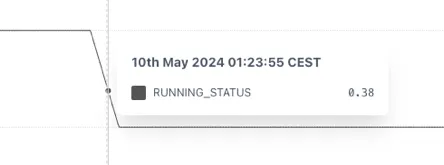
This can be fixed by wrapping the tag in a STEPPED function. Now the change in state properly shown.

2.13.2 STEPPEDRAW: Stepped Raw

The STEPPEDRAW function is identical to the STEPPED function other than it forces the use of Raw data, even if the Trend is set to Interpolated mode.

This is especially useful for reports where one needs to return an accurate total.

Use case

Forcing a TOTALISE calculation to correctly sum a forecast over a month. If the forecast has the following data:

Month	Rate	Monthly Vol.
01-Jan 00:00	1 m3/d	31 m3
01-Feb 00:00	0 m3/d	0 m3

If the Forecast rate is totalised for January without forcing the data to be stepped, then the totalizer will interpolate between 1 and 0 over January and the result will be:

TOTALISE(Rate, MONTH, BEGIN_MONTH, 1d) = 15.5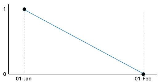

If the Rate is wrapped in a STEPPEDRAW tag it will force the calculation to step the underlying data and the result will be correct.

TOTALISE(STEPPEDRAW(Rate), MONTH, BEGIN_MONTH, 1d) = 31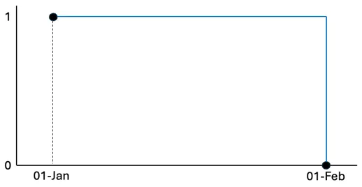

2.13.3 NOBAD: No BAD

The No Bad function removes points from the timeseries that have a “Bad” quality according to the OPC standard[^2] (possible options are Good, Uncertain or Bad) in Raw mode only.

The syntax for a NOBAD function is:

NOBAD(a)

a — any valid timeseries source — see section 2.2

This function has very limited use cases but can help if a tag has randomly incorrect data (i.e. both positive and negative) that cannot be otherwise filtered out.

Because it depends on the raw data, it’s performance can be slower than other functions.

2.13.4 TIMESHIFT

The TIMESHIFT calculation is used when the source data has an incorrect timestamp. This could be because of an incorrectly set timezone or the recording device may have the wrong time. The syntax for a TIMESHIFT function is:

TIMESHIFT(a, offset)

a — any valid timeseries source — see section 2.2

offset — an expression describing how far to shift the data back in time — see below for options

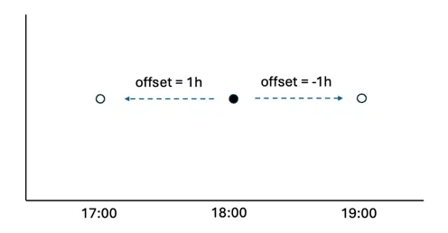
The offset is the amount of time that the source data is away from the time that you want it to be. For example, if a data point is recorded as 06:00 but it should be 07:00 then the data is “1h behind”, so the offset is “-1h” or “-01:00”.

The offset is added to the time range of the data requested so that, if a chart shows data between 12:00 - 14:00 and the TIMESHIFT function has an offset of “1h”, it will return data from the source between 13:00 — 15:00. This has the effect of moving values to the left on a trend. i.e.

Positive values shift data to an earlier point in time.

The offset can be defined in several ways. Positive values shift data to an earlier point in time:

• number of milliseconds (3600000 = 1 hour)

• an exact time definition (1s, 1h, 7d etc.) — see section 2.2 Values can be both positive and negative.

• A time expression in hh:mm or hh:mm:ss. For example, to correct a value that is 2minutes and 14 secs slow you would use -00:02:14

•  java-style durations and periods, e.g. P1D for calendar day, PT24H for exactly 24 hours

• relative time expressions, like “2 hours ago” — see section 2.4.

Examples

Retrieve value of tag at end of previous day:

"calc/TIMESHIFT(calc/TOTALISE2(constants/1, MONTH, BEGIN_MONTH,
1d), **last moment of yesterday**)",

Retrieve value of tag at end of previous day relative to another date

calc/TIMESHIFT(calc/TOTALISE2(constants/1, MONTH, BEGIN_MONTH, 1d), last
moment of yesterday)"

2.13.5 HIGHPASS

The HIGHPASS function applies a filter to a timeseries that lets the high frequencies pass and filters out the low frequencies. The syntax for the HIGHPASS function is:

HIGHPASS(tag, cutoff)

tag - any valid timeseries source - see section 2.2

cutoff - a value in second that defines the cutoff frequency. E.g. 3600 will allow peaks that occur up to an hour apart

Note that

HIGHPASS= tag – LOWPASS(tag, cutoff)

And vice-versa

2.13.5 LOWPASS

The LOWPASS function applies a filter to a timeseries that lets the high frequencies pass and filters out the low frequencies. The syntax for the LOWPASS function is:

LOWPASS(tag, cutoff)

tag - any valid timeseries source – see section 2.2

cutoff - a value in seconds that defines the cutoff frequency. E.g. 3600 filter out peaks that occur less that an hour apart

2.14 Rounding Functions

The Rounding functions all have the syntax

calc/function(tag, x)

Where

tag - any valid timeseries source – see section 2.2

x - a value specifying the rounding operation as appropriate to the function and described in the following sections.

With the exception of the MROUND function, the value of “x” for the rounding operation can be positive or negative. A positive number is the number of places after the decimal point, a negative number is the number of places before the decimal point. I.e. a value of “-1” is equivalent to rounding to the nearest 10.

2.14.1 ROUND

The ROUND function rounds a number to a specified number of digits. It rounds up if the next digit is 5 or greater, and down otherwise. For example,

calc/ROUND(12.345, 2)

would result in 12.35, while

calc/ROUND(12.344, 2)

would result in 12.34.

2.14.2 ROUNDUP

The ROUNDUP function always rounds a number up, away from zero, to the specified number of digits. For example,

calc/ROUNDUP(12.341, 2)

would result in 12.35.

2.14.3 ROUNDDOWN

The ROUNDDOWN function always rounds a number down, towards zero, to the specified number of digits. For example,

calc/ROUNDDOWN(12.349, 2)

would result in 12.34.

2.14.4 MROUND

The MROUND function rounds a number to the nearest specified multiple. For example,

calc/MROUND(12.34, 0.5)

would round to the nearest 0.5, resulting in 12.5.

2.14.5 FLOOR

The FLOOR function rounds a number down to the nearest specified multiple. For example,

calc/FLOOR(12.34, 0.5)

would round down to 12.

2.14.6 CEILING

The CEILING function rounds a number up to the nearest specified multiple. For example

calc/CEILING(12.34, 0.5)

would round up to 12.5.

2.15 Date

2.15.1 EPOCH_MS: Epoch Milliseconds of raw point

EPOCH_MS Returns number of milliseconds, since 1st January 1970, of each [raw]{.underline} point in the underlying series. For current and historical points it gets last timestamp of point before. i.e for interpolated data it will return the timestamp of the last raw point before.

The syntax for an EPOCH_MS function is:

calc/EPOCH_MS(tag)

Examples

Calculate the number of hours between now and the most recent point stored in the tag:

calc/DIV(SUB(date/CURRENT_EPOCH_MS, calc/EPOCH_MS(tag)),3600000)

This calculation first subtracts the EPOCH_MS of the most recent point from the current time, which will return the number of milliseconds difference. This is then divided by 3,600,000, which is the number of milliseconds in an hour.

2.16 Other

2.16.1 POINTINTIME: Point in Time

The Point In Time function returns that value of the source data at a specific point in time. It is only useful for dashboards and will result in a flat line in a trend. The syntax for POINTINTIME is:

POINTINTIME(a, timereference)

a — any valid timeseries source — see section 2.2

timereference — an expression describing how far to shift the data back in time — see below for options

The timereference can be defined in several ways:

• As an offset from now :

  • number of milliseconds (3600000 = 1 hour)

  • an exact time definition (-1s, -1h, -7d etc.) — see section 2.2

  • relative time expressions, like “2 hours ago” — see section 2.4.

• As a point in time :

  • As a timestamp expression in hh:mm or hh:mm:ss. E.g. 00:00 for midnight this morning

  • relative time expressions, like “last moment of yesterday” — see section 2.4.

Examples

To return the value of a tag at 23:59:59.999 the previous day, the POINTINTTIME syntax is:

POINTINTIME(tag, last moment of yesterday)

Return the value of a tag 2 hours ago:

POINTINTIME(tag, -2h)

2.17 Dates Historian

As of build version ei-v6.71.6 in October 2024 there is a new “Dates” historian that returns data about the date. This does not relate to the date of value in a timeseries, but the date as a reference point itself e.g. on the x-axis. For example, when trended the, functions will use the x-axis time. When used to provide a single value in a dashboard the functions will use either “now” in Live Mode or the last point in the requested time window. The available functions in the dates historian are:

Function	Definition
dates/CURRENT_EPOCH_MS	Return wall clock time in epoch ms. The returned units are “epoch ms”.
dates/DAY	Return number of day in month. Points are returned at midnight of the configured timezone.
dates/DAY_OF_MONTH	Return number of day in month. Points are returned at midnight of the configured timezone.
dates/DAY_OF_MONTH_UTC	Return number of day in month. Points are returned at midnight UTC.
dates/DAY_OF_WEEK	Return number of day in week. Monday is 1, and Sunday is 7. Points are returned at midnight of the configured timezone.
dates/DAY_OF_WEEK_UTC	Return number of day in week. Monday is 1, and Sunday is 7. Points are returned at midnight UTC.
dates/DAY_OF_YEAR	Return number of day in year. Points are returned at midnight of the configured timezone.
dates/DAY_OF_YEAR_UTC	Return number of day in year. Points are returned at midnight UTC.
dates/DAY_UTC	Return number of day in month. Points are returned at midnight UTC.
dates/DAYS_IN_MONTH	Return number of days in month.
dates/IS_BEFORE_TODAY	Return 1 if given timestamp is before midnight of today. (i.e. the opposite of IS_TODAY)
dates/IS_TODAY	Return 1 if given timestamp is today. When trended this will always be zero until the time on the x-axis is today.
dates/MONTH	Return number of month in configured timezone.
dates/MONTH_UTC	Return number of month. Points are returned at midnight UTC.
dates/YEAR	Return number of year. Points are returned at midnight of the configured timezone.
dates/YEAR_UTC	Return number of year. Points are returned at midnight UTC.

2.18 Signal Generator Historian (siggen)

The Signal Generator or “siggen” historian is built in and is useful for generating example timeseries or for modifying other timeseries (for example the saw wave can be used to convert a daily forecast into a ramp showing the forecast to that point in the day).

The syntax is (without the spaces):

function amplitude +/- y-offset @ period +/- x-offset (in milliseconds)

e.g. sin10-30@600-3600000 — sinewave of amplitude -10 to 10; offset by -30 (i.e. between -40 and -20); with a period of 600 seconds; offset by -3600000 milliseconds (1 hr)

The function will complete one full cycle within the period.

Function supported are:

• sin (sine)

• cos (cosine)

• saw (saw wave) — useful to modify daily values

• sq (square wave) — useful as an on/off signal

• sc (S-curve)

• rand (random) — repeatable random number